对应代码:03_layout_algebra.cu
纯 host 代码,不需要 GPU。
Layout 不只是一个数据结构,它支持丰富的代数运算:composition(复合)、inverse(逆)、logical_divide(逻辑拆分)、coalesce(合并)等。这些运算是 CuTe 中 MMA partition、Copy partition、坐标变换的理论基础。
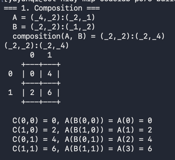
1 2 3 4 5 6 7 8 9 10 11 12 13 14 15 16 17 18 19 20 21 22 23 24 25 26 27 28 29 30 31 32 33 { printf ("=== 1. Composition ===\n" ); auto A = make_layout (make_shape (Int<4 >{}, Int<2 >{}), make_stride (Int<2 >{}, Int<1 >{})); auto B = make_layout (make_shape (Int<2 >{}, Int<2 >{}), make_stride (Int<1 >{}, Int<2 >{})); auto C = composition (A, B); printf (" A = " ); print (A); printf ("\n" ); printf (" B = " ); print (B); printf ("\n" ); printf (" composition(A, B) = " ); print (C); printf ("\n" ); print_layout (C); printf ("\n" ); for (int j = 0 ; j < 2 ; ++j) { for (int i = 0 ; i < 2 ; ++i) { printf (" C(%d,%d) = %d, A(B(%d,%d)) = A(%d) = %d\n" , i, j, int (C (i, j)), i, j, int (B (i, j)), int (A (B (i, j)))); } } printf ("\n" ); }
1
2
3
auto A = make_layout (make_shape (Int<4 >{}, Int<2 >{}), make_stride (Int<2 >{}, Int<1 >{}));auto B = make_layout (make_shape (Int<2 >{}, Int<2 >{}), make_stride (Int<1 >{}, Int<2 >{}));auto C = composition (A, B);
含义 :C(i, j) = A(B(i, j))
执行过程:
先用 B 把二维坐标 (i, j) 映射到一维 index
再用 A 把这个 index 当成一维坐标求 offset
1
2
3
4
B(0,0) = 0 → A(0) = 0 → C(0,0) = 0 B(1,0) = 1 → A(1) = 2 → C(1,0) = 2 B(0,1) = 2 → A(2) = 4 → C(0,1) = 4 B(1,1) = 3 → A(3) = 6 → C(1,1) = 6
用途 :坐标变换的核心操作,inv + compose 实现不同 layout 之间的翻译。
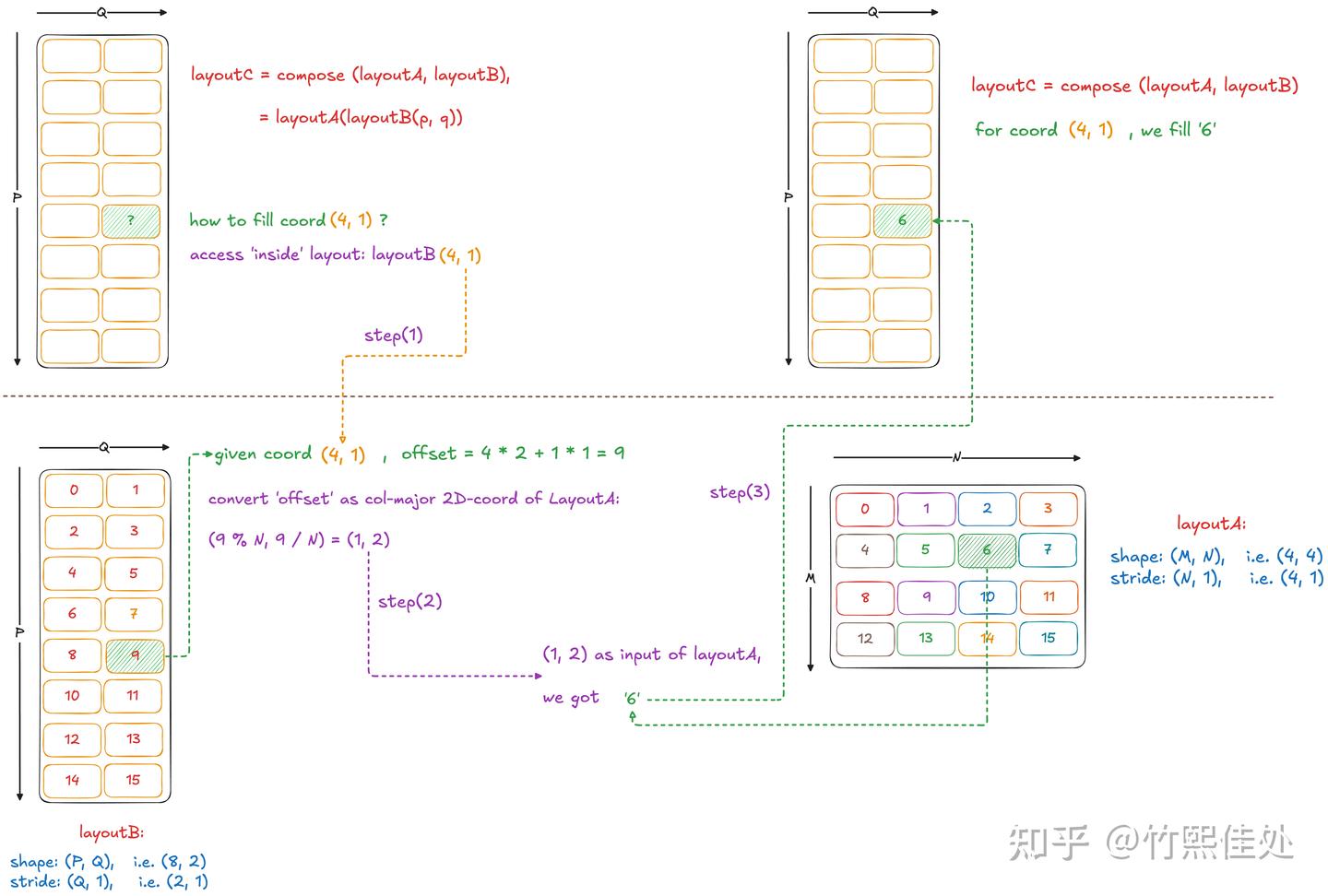
竹佬:事实上,很多初学者会在这里感到困惑,就是没注意到一个 CuTe 中有点反直觉的关键信息:即,对于任意维度的 layout 来说,其输入总是可以兼容 1D 坐标的,这个 1D 坐标会根据这个 layout 的 shape,按照 col-major 的方式来转换为多维坐标,并且这个转换和 stride 无关。
以 layoutA 为例,其 shape 为 (M, N):
1D 坐标 可通过如下公式转换为 2D 坐标: , ;再将转换后的 (m, n) 传入 layoutA,计算得到 (其中 、 为 layoutA 的 stride)。
整个 compose 的计算过程可以展示
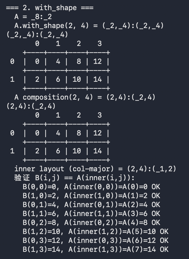
1 2 3 4 5 6 7 8 9 10 11 12 13 14 15 16 17 18 19 20 21 22 23 24 25 26 27 28 29 30 31 32 33 34 35 36 { printf ("=== 2. with_shape ===\n" ); auto A = make_layout (Int<8 >{}, Int<2 >{}); auto B = A.with_shape (make_shape (Int<2 >{}, Int<4 >{})); auto C = composition (A, make_layout (make_shape (2 , 4 ))); printf (" A = " ); print (A); printf ("\n" ); printf (" A.with_shape(2, 4) = " ); print (B); printf ("\n" ); print_layout (B); printf (" A composition(2, 4) = " ); print (C); printf ("\n" ); print_layout (C); auto inner = make_layout (make_shape (2 , 4 )); printf (" inner layout (col-major) = " ); print (inner); printf ("\n" ); printf (" 验证 B(i,j) == A(inner(i,j)):\n" ); for (int j = 0 ; j < 4 ; ++j) { for (int i = 0 ; i < 2 ; ++i) { int inner_val = int (inner (i, j)); int a_val = int (A (inner_val)); int b_val = int (B (i, j)); printf (" B(%d,%d)=%d, A(inner(%d,%d))=A(%d)=%d %s\n" , i, j, b_val, i, j, inner_val, a_val, b_val == a_val ? "OK" : "FAIL" ); } } printf ("\n" ); }
1
2
auto A = make_layout (Int<8 >{}, Int<2 >{}); auto B = A.with_shape (make_shape (Int<2 >{}, Int<4 >{}));
with_shape 等价于 composition(A, make_layout(shape)):
1 2 auto B = composition (A, make_layout (make_shape (2 , 4 )));
原理 :make_layout(make_shape(2, 4)) 创建 col-major layout (2,4):(1,2),然后串联:
1
2
3
4
5
6
7
B(i,j) = A(inner(i,j)) inner = (2,4):(1,2) col-major inner(0,0)=0 → A(0)=0 inner(1,0)=1 → A(1)=2 inner(0,1)=2 → A(2)=4 ...
用途 :把一维 layout 重新解释为多维视图,不改变底层的 offset 映射规则。
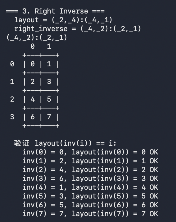
1 2 3 4 5 6 7 8 9 10 11 12 13 14 15 16 17 18 19 20 21 22 23 24 { printf ("=== 3. Right Inverse ===\n" ); auto layout = make_layout (make_shape (Int<2 >{}, Int<4 >{}), make_stride (Int<4 >{}, Int<1 >{})); auto inv = right_inverse (layout); printf (" layout = " ); print (layout); printf ("\n" ); printf (" right_inverse = " ); print (inv); printf ("\n" ); print_layout (inv); printf ("\n" ); printf (" 验证 layout(inv(i)) == i:\n" ); for (int i = 0 ; i < size (inv); ++i) { printf (" inv(%d) = %d, layout(inv(%d)) = %d %s\n" , i, int (inv (i)), i, int (layout (inv (i))), int (layout (inv (i))) == i ? "OK" : "FAIL" ); } printf ("\n" ); }
1
2
auto layout = make_layout (make_shape (Int<2 >{}, Int<4 >{}), make_stride (Int<4 >{}, Int<1 >{}));auto inv = right_inverse (layout);
定义 :layout(inv(i)) == i 对所有 i < size(inv) 成立。
Inverse 的本质 :把 layout 的箭头反过来。Layout 是 index → offset,inverse 是 offset → index。
构造过程 (以 (2,4):(4,1) 为例):
按 stride 升序排列维度:stride=1(shape=4)在前,stride=4(shape=2)在后
排序后 shape = (4, 2)
inverse 的 stride 用 col-major 前缀积 = (1, 4)
最终结果 (4, 2):(1, 4)
验证 :
1
2
3
4
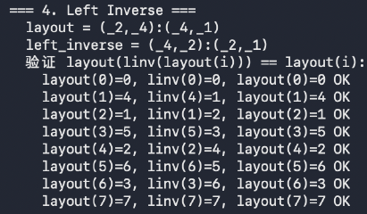
inv(0)=0, layout(0)=0 ✓ inv(1)=2, layout(2)=1 ✓ inv(2)=4, layout(4)=2 ✓ ...
1 2 3 4 5 6 7 8 9 10 11 12 13 14 15 16 17 18 19 20 21 22 23 24 25 { printf ("=== 4. Left Inverse ===\n" ); auto layout = make_layout (make_shape (Int<2 >{}, Int<4 >{}), make_stride (Int<4 >{}, Int<1 >{})); auto linv = left_inverse (layout); printf (" layout = " ); print (layout); printf ("\n" ); printf (" left_inverse = " ); print (linv); printf ("\n" ); printf (" 验证 layout(linv(layout(i))) == layout(i):\n" ); for (int i = 0 ; i < size (layout); ++i) { int li = layout (i); int linv_li = linv (li); int result = layout (linv_li); printf (" layout(%d)=%d, linv(%d)=%d, layout(%d)=%d %s\n" , i, li, li, linv_li, linv_li, result, result == li ? "OK" : "FAIL" ); } printf ("\n" ); }
1
2
auto layout = make_layout (make_shape (Int<2 >{}, Int<4 >{}), make_stride (Int<4 >{}, Int<1 >{}));auto linv = left_inverse (layout);
定义 :layout(linv(layout(i))) == layout(i) 对所有 i < size(layout) 成立。
比 right_inverse 更宽松——即使 layout 不是双射(有多对一的情况)也能用。
在坐标变换中的用途 :用 left_inverse 更安全,因为 MMA/Copy 的 layout 可能不是完美双射。
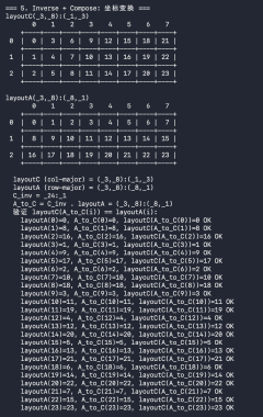
1 2 3 4 5 6 7 8 9 10 11 12 13 14 15 16 17 18 19 20 21 22 23 24 25 26 27 28 29 30 31 32 33 34 35 36 37 { printf ("=== 5. Inverse + Compose: 坐标变换 ===\n" ); auto layoutC = make_layout (make_shape (Int<3 >{}, Int<8 >{}), make_stride (Int<1 >{}, Int<3 >{})); auto layoutA = make_layout (make_shape (Int<3 >{}, Int<8 >{}), make_stride (Int<8 >{}, Int<1 >{})); printf ("layoutC" ); print_layout (layoutC); printf ("\n" ); printf ("layoutA" ); print_layout (layoutA); printf ("\n" ); auto C_inv = left_inverse (layoutC); auto A_to_C = composition (C_inv, layoutA); printf (" layoutC (col-major) = " ); print (layoutC); printf ("\n" ); printf (" layoutA (row-major) = " ); print (layoutA); printf ("\n" ); printf (" C_inv = " ); print (C_inv); printf ("\n" ); printf (" A_to_C = C_inv . layoutA = " ); print (A_to_C); printf ("\n" ); printf (" 验证 layoutC(A_to_C(i)) == layoutA(i):\n" ); for (int i = 0 ; i < size (layoutA); ++i) { printf (" layoutA(%d)=%d, A_to_C(%d)=%d, layoutC(A_to_C(%d))=%d %s\n" , i, int (layoutA (i)), i, int (A_to_C (i)), i, int (layoutC (A_to_C (i))), int (layoutC (A_to_C (i))) == int (layoutA (i)) ? "OK" : "FAIL" ); } printf ("\n" ); }
1
2
3
4
5
auto layoutC = make_layout (make_shape (Int<3 >{}, Int<8 >{}), make_stride (Int<1 >{}, Int<3 >{}));auto layoutA = make_layout (make_shape (Int<3 >{}, Int<8 >{}), make_stride (Int<8 >{}, Int<1 >{}));auto C_inv = left_inverse (layoutC);auto A_to_C = composition (C_inv, layoutA);
目标 :给定 A 坐标系的 index,找到 C 坐标系的 index,使得两者指向同一个物理 offset。
原理 :利用物理地址做桥梁,分两步走:
1 index_A --layoutA--> offset --C_inv--> index_C
即 A_to_C(i) = C_inv(layoutA(i)),composition 自动完成这个串联。
具体数字 :
1
2
3
4
5
6
问:A 的 1 号在 C 里是几号? 第一步:layoutA(1) = 8 ← A 的 1 号在物理地址 8 第二步:C_inv(8) = 8 ← 物理地址 8 在 C 里是 8 号 验证:layoutC(8) = 8 ✓ 同一个物理位置
Shape 整除性要求 :composition(C_inv, layoutA) 要求 layoutA 的 shape 因子和 C_inv 的 shape 因子之间有整除关系。如果不满足,编译报 “Shape Divisibility Condition” 错误。
实际用途 :MMA 输出的 C-layout 寄存器 → Copy 需要的 A-layout 寄存器,就是用这个坐标变换实现的(retile_D)。
竹佬:
在笔者刚开始接触 CuTe 时,常常会困惑于一件事:这些 layout 代数究竟有什么用?大家对于 CuTe 官方文档吐槽也主要因为其完全没有前后联系的抛出一堆概念和代数运算,然后指望用户自己从庞大的代码库中理解其用法,人为制造出一条陡峭到天上的学习曲线。
作为一篇写给大家看的教程,我们不急于输出更多的概念,先结合 Flash atten v2 中 A-layout 到 C-layout 转换这个例子,来感受一下 layout compose & inverse 的用法和其蕴含的潜力。
我们知道在 Flash atten v2 的实现中,核心是 P = Q @ K.T 以及 O = P @ V 两个矩阵连乘(为简化说明,我们先忽略 softmax 的运算),在这个过程中 P 即是 QK 矩阵乘的输出,此时其符合 mma accumulator tensor 的 layout;也是 PV 矩阵乘的输入,此时其又需要符合 mma A tensor 的 layout。我们知道,tiled mma 的 layout 要求 A 和 C tensor 的 layout 是不同的,直接将 C 作为 A tensor 输入到 cute::gemm 函数中会编译报错。那么需要怎么对 C 进行转换呢?
我们从 C = A @ B.T 这样一个简单的例子,延伸出一个简化的矩阵连乘来说明。即,我们想完成 C = A @ B.T,D = C @ B.T 这样一个计算:
1
2
3
4
5
6
7
8
9
10
11
12
13
14
15
16
17
18
19
20
21
22
23
24
25
26
27
28
29
30
31
32
33
34
35
36
37
38
39
40
41
42
43
44
45
46
47
48
49
50
51
52
53
54
55
56
57
58
template <typename T, int kTileM, int kTileN, int kTileK, typename TiledMMA>__global__ void simple_kernel (T *Cptr, const T *Aptr, const T *Bptr, int m, int n, int k) Tensor A = make_tensor (make_gmem_ptr (Aptr), make_shape (m, k), make_stride (k, Int<1 >{})); Tensor B = make_tensor (make_gmem_ptr (Bptr), make_shape (n, k), make_stride (k, Int<1 >{})); Tensor C = make_tensor (make_gmem_ptr (Cptr), make_shape (m, n), make_stride (n, Int<1 >{})); int ix = blockIdx.x; int iy = blockIdx.y; Tensor gA = local_tile (A, make_tile (Int<kTileM>{}, Int<kTileK>{}), make_coord (iy, _)); Tensor gB = local_tile (B, make_tile (Int<kTileN>{}, Int<kTileK>{}), make_coord (ix, _)); Tensor gC = local_tile (C, make_tile (Int<kTileM>{}, Int<kTileN>{}), make_coord (iy, ix)); TiledMMA tiled_mma; auto thr_mma = tiled_mma.get_slice (threadIdx.x); auto tgA_g2r = thr_mma.partition_A (gA); auto tgB_g2r = thr_mma.partition_B (gB); auto tgC_g2r = thr_mma.partition_C (gC); auto trA_mma = thr_mma.partition_fragment_A (gA (_, _, 0 )); auto trB_mma = thr_mma.partition_fragment_B (gB (_, _, 0 )); auto trC_mma = thr_mma.partition_fragment_C (gC (_, _)); auto trD_mma = thr_mma.partition_fragment_C (gC (_, _)); clear (trC_mma); clear (trD_mma); int num_tile_k = size <2 >(gA); #pragma unroll 1 for (int itile = 0 ; itile < num_tile_k; ++itile) { cute::copy (tgA_g2r (_, _, _, itile), trA_mma); cute::copy (tgB_g2r (_, _, _, itile), trB_mma); cute::gemm (tiled_mma, trC_mma, trA_mma, trB_mma, trC_mma); auto trC_as_A_mma = trC_mma; cute::gemm (tiled_mma, trD_mma, trC_as_A_mma, tBrB_mma, trD_mma); } }
以 16x8x16 fp16 mma atom 为例,trC 作为 accumulator layout 为 ((2, 2), MMA_M, MMA_N),而下一次 gemm 所需要其作为 A-tensor,需要其 layout 为 ((2, 2, 2), MMA_M, MMA_N / 2)。
二者的数据本身是完全一致的,因此我们需要对 trC layout 进行一次变换。熟悉 flash atten v2 的读者可能已经发现,Tri-dao 在其实现中使用了 logical_divide 对 layout 在几何层面上进行了一次重排,我们将其过程拆解出来如下:
1 2 3 4 5 6 7 8 9 10 11 12 13 14 15 16 17 18 19 20 21 22 23 cute::gemm (tiled_mma, trC_mma, trA_mma, trB_mma, trC_mma); auto acc_layout_div = logical_divide ( trC_mma.layout (), Shape<Underscore, Underscore, _2>{}); auto a_layout = make_layout ( make_layout (get <0 >(acc_layout_div), get <2 , 0 >(acc_layout_div)), get <1 >(acc_layout_div), get <2 , 1 >(acc_layout_div)); auto trC_as_A_mma = make_tensor (trC_mma.data (), a_layout);cute::gemm (tiled_mma, trD_mma, trC_as_A_mma, tBrB_mma, trD_mma);
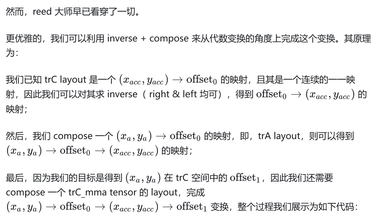
1 2 3 4 5 6 7 8 9 10 11 12 13 14 15 16 17 18 19 20 21 22 23 24 25 26 27 28 cute::gemm (tiled_mma, trC_mma, trA_mma, trB_mma, trC_mma); auto C_tensor_for_partition = make_tensor_like (gC (_, _));auto trC_as_A_layout = thr_mma.partition_A (C_tensor_for_partition).layout ();auto trC_as_C_layout = thr_mma.partition_C (C_tensor_for_partition).layout (); auto acc_layout_inv = left_inverse (trC_as_C_layout);auto a_layout_algebra = acc_layout_inv.compose (trC_as_A_layout);auto trC_as_A_mma = trC_mma.compose (a_layout_algebra);cute::gemm (tiled_mma, trD_mma, trC_as_A_mma, tBrB_mma, trD_mma);
我们建议感兴趣的读者可以尝试跑通这个例子,并验证一下 tri-dao 和 reed 两者方法的结果,并尝试在更多的 mma 规格上测试,来感受 layout 代数所带来的语义上的便利性。
详细解析请见附录
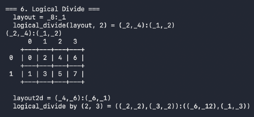
1 2 3 4 5 6 7 8 9 10 11 12 13 14 15 16 17 18 19 20 21 22 23 24 { printf ("=== 6. Logical Divide ===\n" ); auto layout = make_layout (Int<8 >{}, Int<1 >{}); auto divided = logical_divide (layout, Int<2 >{}); printf (" layout = " ); print (layout); printf ("\n" ); printf (" logical_divide(layout, 2) = " ); print (divided); printf ("\n" ); print_layout (divided); printf ("\n" ); auto layout2d = make_layout (make_shape (Int<4 >{}, Int<6 >{}), make_stride (Int<6 >{}, Int<1 >{})); auto div2d = logical_divide (layout2d, make_tile (Int<2 >{}, Int<3 >{})); printf (" layout2d = " ); print (layout2d); printf ("\n" ); printf (" logical_divide by (2, 3) = " ); print (div2d); printf ("\n" ); printf ("\n" ); }
1
2
3
auto layout = make_layout (Int<8 >{}, Int<1 >{});auto divided = logical_divide (layout, Int<2 >{});
含义 :把一个维度拆成 (tile_size, num_tiles)。
1
2
3
4
5
6
7
8 个元素,按 2 拆: (2, 4):(1, 2) | | | | | | | └── num_tiles 的 stride = tile_size × 原始 stride = 2 | | └── tile 内的 stride = 原始 stride = 1 | └── num_tiles = 8/2 = 4 └── tile_size = 2
多维版本 :
1
2
3
auto layout2d = make_layout (make_shape (Int<4 >{}, Int<6 >{}), make_stride (Int<6 >{}, Int<1 >{}));auto div2d = logical_divide (layout2d, make_tile (Int<2 >{}, Int<3 >{}));
用途 :local_tile 内部就是用 logical_divide 实现的。在 MMA 中,logical_divide 用于把 fragment 的 MMA_N 维度拆成 (2, MMA_N/2) 来做 C→A layout 转换。
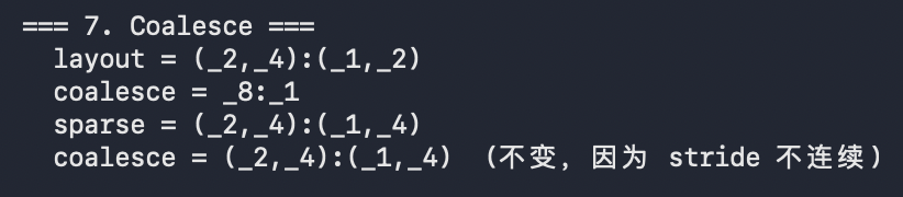
1 2 3 4 5 6 7 8 9 10 11 12 13 14 15 16 17 18 19 20 { printf ("=== 7. Coalesce ===\n" ); auto layout = make_layout (make_shape (Int<2 >{}, Int<4 >{}), make_stride (Int<1 >{}, Int<2 >{})); auto coalesced = coalesce (layout); printf (" layout = " ); print (layout); printf ("\n" ); printf (" coalesce = " ); print (coalesced); printf ("\n" ); auto sparse = make_layout (make_shape (Int<2 >{}, Int<4 >{}), make_stride (Int<1 >{}, Int<4 >{})); auto sparse_c = coalesce (sparse); printf (" sparse = " ); print (sparse); printf ("\n" ); printf (" coalesce = " ); print (sparse_c); printf (" (不变,因为 stride 不连续)\n" ); printf ("\n" ); }
1
2
3
auto layout = make_layout (make_shape (Int<2 >{}, Int<4 >{}), make_stride (Int<1 >{}, Int<2 >{}));auto coalesced = coalesce (layout);
含义 :把可以合并的相邻维度合并成一个。
合并条件 :stride[i+1] == stride[i] × shape[i](即两个维度在内存中是连续的)。
1
2
(2, 4):(1, 2) → stride[1]=2 == stride[0]×shape[0]=1×2 ✓ → 合并为 (8):(1) (2, 4):(1, 4) → stride[1]=4 != stride[0]×shape[0]=1×2 ✗ → 不合并,保持原样
用途 :简化 layout,去掉多余维度,有时能让后续操作更高效。
1
2
3
4
5
6
composition(A, B) → C(i,j) = A(B(i,j)) 函数复合 with_shape(shape) → composition(self, col_major) 重塑输入空间 right_inverse(L) → inv, 满足 L(inv(i)) = i 编号→offset 的反函数 left_inverse(L) → inv, 满足 L(inv(L(i))) = L(i) 更宽松的反函数 logical_divide(L, T) → 把维度拆成 (tile, num_tiles) 切 tile 的基础 coalesce(L) → 合并连续维度 简化 layout
同一块数据 ,两种不同的 layout 给出不同的"坐标系"。坐标变换就是从一种坐标系转换到另一种坐标系 ,使得两个坐标指向同一个物理位置。
例如同一块 24 个元素的数据:
1
2
layoutC = (3,8):(1,3) col-major → layoutC(i) = offset layoutA = (3,8):(8,1) row-major → layoutA(i) = offset
物理位置 offset=8 的元素,在两种坐标系里的 index 不同:
layoutC 眼里:index=8 → layoutC(8) = 8
layoutA 眼里:index=1 → layoutA(1) = 8
同一个元素,A 叫它 “1号”,C 叫它 “8号”。
A_to_C = composition(C_inv, layoutA) 就是翻译表:
1
2
A_to_C(1) = 8 → A 坐标系的 1 号 = C 坐标系的 8 号 验证:layoutC(A_to_C(1)) = layoutC(8) = 8 = layoutA(1) ✓ 同一个 offset
实际用途 :MMA 指令算完的结果在寄存器里,以 C-layout 编号;写回 smem/gmem 时 Copy 操作需要 A-layout 编号。坐标变换让同一组寄存器在 MMA 和 Copy 两种视角之间正确切换,这就是 retile_D 做的事。不做这个变换,MMA 的结果就会写错位置。
Inverse 的本质:把 layout 的箭头方向反过来。
Layout 是一个函数:编号 → 物理地址。Inverse 就是反过来:物理地址 → 编号。
1
2
layoutC: index_C → offset (查号簿:名字→电话) C_inv: offset → index_C (反查号簿:电话→名字)
为什么 inv + compose 能算出坐标变换?
我们要的是:给一个 A 的编号,找到 C 的编号,使得它们指向同一个物理地址。分两步走:
1
2
第一步:layoutA 把 A 编号翻译成物理地址 index_A → offset 第二步:C_inv 把物理地址翻译成 C 编号 offset → index_C
串起来(composition)就是:
1 index_A --layoutA--> offset --C_inv--> index_C
两种 layout 虽然编号方式不同,但底层共享同一个物理地址空间,物理地址就是天然的中转站。
用具体数字走一遍(layoutA = (3,8):(8,1), layoutC = (3,8):(1,3)):
1
2
3
4
5
6
7
8
问:A 的 1 号元素,在 C 里是几号? 第一步:layoutA(1) = 8 ← A 的 1 号在物理地址 8 第二步:C_inv(8) = 8 ← 物理地址 8 在 C 里是 8 号 结论:A 的 1 号 = C 的 8 号 验证:layoutC(8) = 8 ✓ 确实指向同一个物理地址
图示:
1
2
3
4
5
6
7
layoutA C_inv index_A ---------> offset -----------> index_C 1 ----------> 8 -----------> 8 layoutC index_C ---------> offset 8 ----------> 8 ✓ 同一个物理位置
以 Flash Attention 为例,计算 P = Q @ K.T,然后 D = P @ V:
第一个 GEMM 的输出 P 存在累加器寄存器里,其 layout 是 C-layout:((2,2), MMA_M, MMA_N)
第二个 GEMM 需要 P 作为输入 A,要求 A-layout:((2,2,2), MMA_M, MMA_N/2)
数据完全一样,只是同一组寄存器需要用不同的 layout 去解读
用 logical_divide 手动把 MMA_N 维度拆成 (2, MMA_N/2),然后手动重组:
1
2
3
4
5
6
7
8
auto acc_layout_div = logical_divide ( trC_mma.layout (), Shape<Underscore, Underscore, _2>{}); auto a_layout = make_layout ( make_layout (get <0 >(acc_layout_div), get <2 , 0 >(acc_layout_div)), get <1 >(acc_layout_div), get <2 , 1 >(acc_layout_div)); auto trC_as_A_mma = make_tensor (trC_mma.data (), a_layout);
需要手动理解两种 layout 的结构差异,换 MMA 规格就得重写。
利用 inverse + compose 自动推导坐标变换:
1 2 3 4 auto C_tensor_for_partition = make_tensor_like (gC (_, _));auto trC_as_A_layout = thr_mma.partition_A (C_tensor_for_partition).layout ();auto trC_as_C_layout = thr_mma.partition_C (C_tensor_for_partition).layout ();
对同一块 (kTileM, kTileN) 数据,分别用 partition_A 和 partition_C 切,得到两种 layout。
两者映射到的 offset 空间是同一个(同一块数据的元素编号),只是坐标系不同。
1 2 3 auto acc_layout_inv = left_inverse (trC_as_C_layout);
1 2 3 4 5 6 auto a_layout_algebra = acc_layout_inv.compose (trC_as_A_layout);
1 2 3 4 5 auto trC_as_A_mma = trC_mma.compose (a_layout_algebra);
Tensor 的 compose 实现(tensor_impl.hpp:284):
1
2
3
auto compose (Layouts const &... layouts) return make_tensor (data (), layout ().compose (layouts...)); }
data() 原封不动传过去(同一个指针/同一组寄存器),只对 layout 做了 compose 变换。
数据没变,变的是"门牌号"——同一组寄存器用新的坐标映射去索引。
1
2
3
4
5
6
7
8
9
10
partition_C 得到: (x_c, y_c) -> offset ... (1) left_inverse: offset -> (x_c, y_c) ... (1)^{-1} partition_A 得到: (x_a, y_a) -> offset ... (2) compose (1)^{-1} . (2): (x_a, y_a) -> (x_c, y_c) ... 坐标变换 trC_mma 的 layout: (x_c, y_c) -> 寄存器 ... (3) 最终 compose (3) . (1)^{-1} . (2): (x_a, y_a) -> 寄存器 ... 目标达成
Tri-Dao
Reed
思路
手动拆维度、重组
代数变换:inverse + compose
是否需要了解具体 layout 结构
需要
不需要,自动推导
换 MMA 规格
可能要改代码
通用,不用改